Crime Data Exploration with Python3, Numpy, and Pandas: Part 1

July 13, 2019    |    Data Exploration    |    Pandas    |    Python

Overview

Data is everywhere. Crime is too. The FBI runs a program called Uniform Crime Reporting (UCR) Program that collects crime data from ~18,000 agencies all over the United States. This database is a gold mine of interesting statistics about crime in the United States. Follow along and learn about how you can use Python to analyze this data. My hope is that you learn from this article and then go do some data exploration on your own.

Full Source code: https://github.com/rbk/Crime-Data-Analysis

Data Tools We’ll Use

Data scientists are known to use Python for machine learning and data cleaning. What you may not know is that there are some fantastic libraries in Python for performing operations on JSON, CSV, and other data types.

You are going to fall in love with Pandas very soon. No not the cute cuddly pandas you see at the zoo, Pandas the Python package. Pandas is a library that makes dealing with massive arrays of data a breeze as you will see in the next section. Pandas is built on top of Numpy. I recommend checking them both out:

• https://pandas.pydata.org/
• https://www.numpy.org/

Download the Dataset

Grab the dataset to begin. You can use whichever method is easiest for you to download the dataset. Here is the URI of the dataset we will be working with:

http://s3-us-gov-west-1.amazonaws.com/cg-d4b776d0-d898-4153-90c8-8336f86bdfec/estimated_crimes.csv

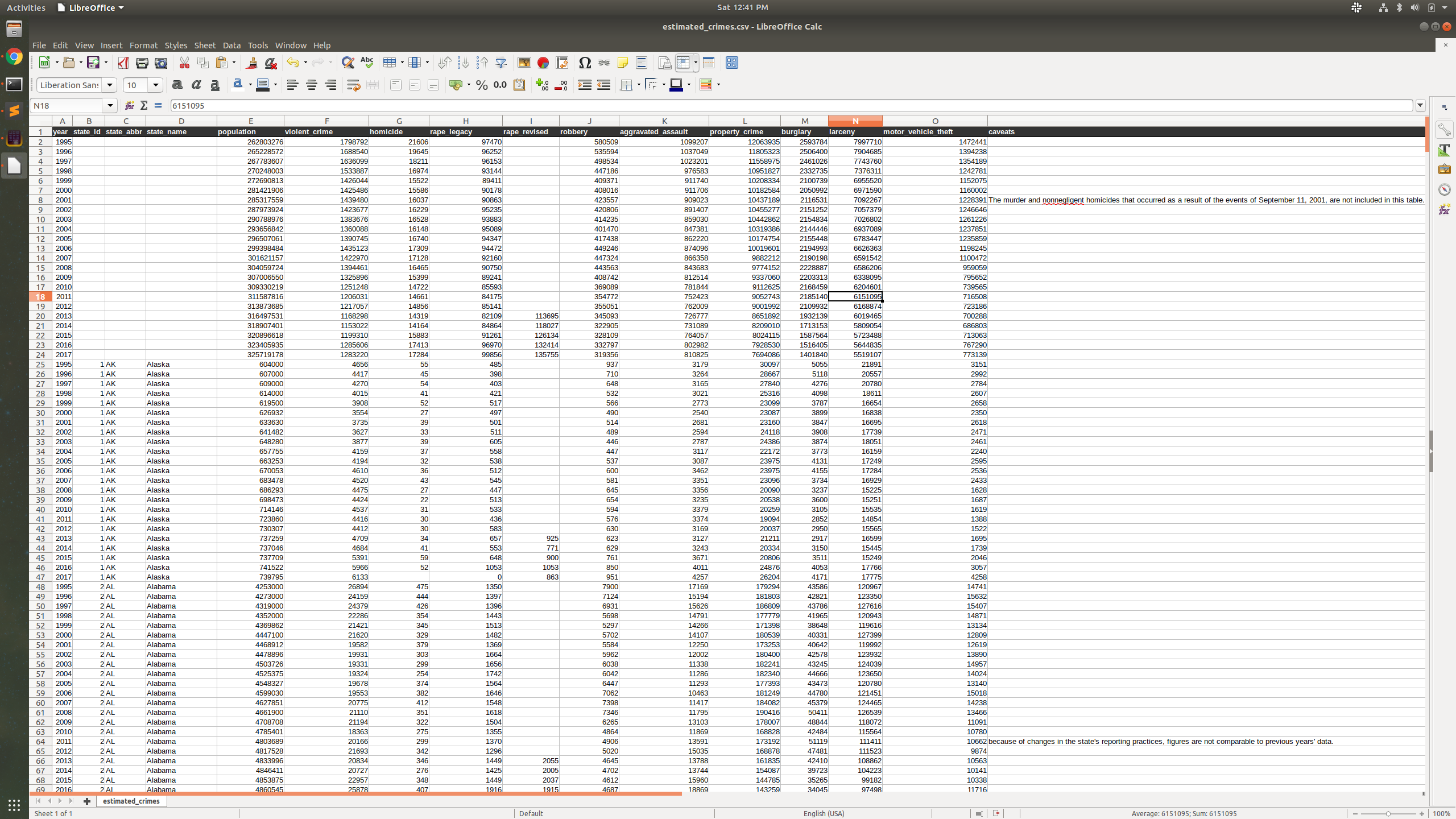
This dataset contains the estimated counts of criminal incidents reported from 1995 to 2017 in all the United States.

Before diving into the code there is one more thing…disclaimer time.

Disclaimer About Drawing Conclusions from this Crime dataset

The crime dataset is a compilation of incident reports over time. The term “Crime Rate” is the number of crimes per person in a given population. It is important to note that this doesn’t take into account the hundreds of risk factors associated with the safety of a city or state. For example, New Mexico may have a higher crime rate than average, but statistically, that doesn’t mean New Mexico is a dangerous place to live. The data doesn’t take into account the population density, economic conditions, employment rates, and the effective strength of the police force¹.

Furthermore, you cannot just assume that a certain state is safer because the crime rate is below average. The reason this claim is invalid is that crime in certain areas could just not be reported because of the crime itself.

Alright, enough of the disclaimer…

Time to Code!

Fire up your IDE or editor or Jupyter Notebook ladies and gents. We are going in line by line. You should have a folder with a CSV file called estimated_crimes.csv. In this folder, you need a Python file. I usually use main.py. This code will be in Python3. You’ll also need to pip install pandas:

pip install pandas

Objective

In the following steps, we will transform the CSV file from the FBI into a new CSV with new columns that help us visually understand the data. Specifically, we are going to determine the average crime rate on the national level and then compare each US state’s crime rate to show the percentage difference relative to the national average.

Step 1: Load the CSV into a Pandas Dataframe

The first thing we need to do is get control of our data. In its raw format, it is a little awkward to work with. Pandas is the tool of choice for transforming data into different forms that are easier to work with.

The first trick you must know about Pandas when working with CSV files is the amazing read_csv function. The read_csv function will load any CSV file into a Pandas Dataframe. From this dataframe we can use all kind of pandas functions to manipulate and query the data.

import pandas

# Read the CSV into a Dataframe
data = pandas.read_csv('estimated_crimes.csv')

Once the data is read into a variable we can use the head function to print the first 5 rows of the dataframe:

# Print the first 5 lines of the dataframe
print(data.head())

Output

Now before moving on, lets remove the columns of the data we don’t need right now. To do this, read the CSV with the usecols option. usecols tells the read function to only use a specified list of columns:

import pandas

# Which columns to use
columns = ['year', 'state_name', 'population', 'violent_crime', 'property_crime']

# Get the data into a dataframe from csv
data = pandas.read_csv('estimated_crimes.csv', usecols=columns)

Now when you print the data it is easier to visualize.

# Print the first 5 lines of the dataframe
print(data.head())

Output

Step 2: Filter Data

Now that you have the data in a dataframe you have unleashed the power of Pandas! The second trick of Pandas is the query function. With the query function we can filter our CSV file to only contain rows for a specific year.

Using our dataframe from above:

data = data.query('year == 2017')

If that doesn’t make you excited to use pandas I don’t know what will. After running this query function our data should only contain rows in which the year column is 2017.

Another filter we need to add is to remove row in which the state column is null. In this particular CSV the top rows are the compiled national stats, so the state column is not filled out. We can filter these rows by using the pandas notnull function:

data = data[data['state_name'].notnull()]

Any row in which the state column is null or NaN, will be removed from the dataframe.

Step 3: Add new data columns with apply

Now that we have the data cleaned up. We’ll add three columns. Using the pandas apply function we can create new columns in the data in two steps.

The first step is to define your function. This function will take each row from the dataframe. For example, the following function will calculate the crimes per 1000 people in each row.

def crime_per_capita(row, number_of_people):
    total_crimes = row['violent_crime'] + row['property_crime']
    population = row['population']
    count = (total_crimes/population)*number_of_people
    return count

Our dataframe can now use this function to create a new column by using apply:

data['crime_per_1000'] = data.apply(crime_per_capita, args=(1000,), axis=1)
print(data.head())

Running print head will show a new column with the number of crimes for every 1000 people.

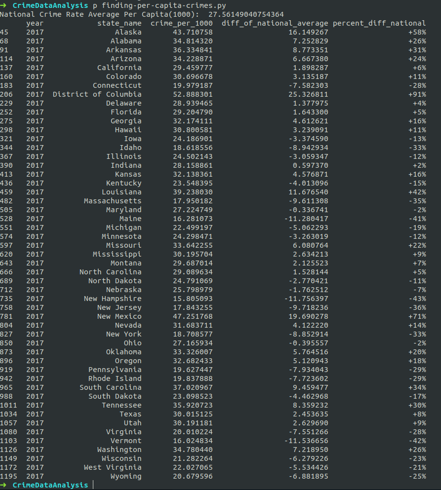
Next we will compute the national crime rate, then use the national crime rate to compare each individual states crime rate. Once we compute the percentage difference of the national average crime rate to each US State, we will be able to quickly see the differences in crime rates across the US.

# 1 Get National Average
total_population = data['population'].sum()
total_crimes =+ data['violent_crime'].sum() + data['property_crime'].sum()
national_average_per_cap = (total_crimes/total_population)*1000

# 2.0 Add column of diff to national average
def compute_diff(row):
    diff = row['crime_per_1000'] - national_average_per_cap
    return diff

data['diff_of_national_average'] = data.apply(compute_diff, axis=1)

# 2.1 Add column of percent diff compared to national average
def compute_percent(row):
    percent = (row['crime_per_1000']/national_average_per_cap)*100
    if percent > 100:
        return "+" + str(int(percent-100)) + "%"
    return "-" + str(100 - int(percent)) + "%"

data['percent_diff_national'] = data.apply(compute_percent, axis=1)

Drawing Conclusions

From the data above we can see that:

• Ohio and Maryland have the lowest crime rates 2% below the average. This means that there we fewer crimes reported for every 1000 people than the national average.
• Maryland has the fewest crimes per capita in 2017.
• The crime rate in the District of Columbia is nearly twice the national average (+91% above the national average).

The possibilities of data exploration are endless with this dataset and many others.
Just keep in mind that you should take heed to the disclaimer before making assumptions about safety on just one dimensinal data like this. There are hundreds of factors that determine the actual safety of a city or neighborhood.

To conclude, we looked at a dataset from the FBI UCR website called “estimated_crimes.csv”. We used the Pandas python library to filter and transform the data so that it could be read easier. We then came up with a few conclusions about the data.

Stay tuned for Part 2 where we dive deeper into the Crime datasets.

Resources and References

• [1] https://crime-data-explorer.fr.cloud.gov/explorer/state/california/crime/1995/2017
• https://www.fbi.gov/services/cjis/ucr
• https://crime-data-explorer.fr.cloud.gov/downloads-and-docs
• https://definitions.uslegal.com/c/crime-rate/ -> “Population-based rates fail to take into account variations in risk.”